Occasionally Faulty Sensor

Jacob Brazeal asked an interesting question on his blog: A puzzle of two unreliable sensors. I have been spending some time learning R recently, and decided to play around with this problem a bit more, with a focus on visualizing what’s going on.

His puzzle goes like this: Say that you have two sensors, \(A\) and \(B\), both observing some variable \(P\).

• \(P\) is a random number between 0 and 1.
• \(A\) takes the average of \(P\) and a random number between 0 and 1 (random uniform noise).
• \(B\) is occasionally faulty. Half the time, \(B\) will perfectly report \(P\). The other half of the time, \(B\) will report a useless random number between 0 and 1.

Precisely:

It turns out that both \(A\) and \(B\) seem to predict \(P\) with the same mean absolute (L1) error of approximately 0.16666, but the average of them (\(\frac{A + B}{2}\)) slightly improves on their mean absolute error to around 0.15275. Even stranger, a weighted average giving slight emphasis to \(A\) (i.e, \(0.58A + 0.42B\)) further reduces the mean absolute error to 0.15234.

So what is going on? And can we gain any intuition for this problem?

Let’s generate a large number of samples, maintaining values of \(A, B, P\) and also a FAULTY variable (for ease of inspection):

|   | P       | FAULTY | A       | B       |
|---+---------+--------+---------+---------|
| 1 | 0.89670 | TRUE   | 0.57926 | 0.43178 |
| 2 | 0.26551 | FALSE  | 0.44493 | 0.26551 |
| 3 | 0.37212 | TRUE   | 0.22141 | 0.28037 |
| 4 | 0.57285 | FALSE  | 0.30797 | 0.57285 |
| 5 | 0.90821 | FALSE  | 0.61127 | 0.90821 |
| 6 | 0.20168 | TRUE   | 0.36078 | 0.18898 |

Now let’s recover the results from Jacob’s work:

d |>
    summarize(
        A_MAE = mean(abs(A - P)),
        B_MAE = mean(abs(B - P)),
        midpoint_MAE = mean(abs((A + B) / 2 - P)),
        `58pct_A_MAE` = mean(abs((0.58 * A + 0.42 * B - P))),
        A_MSE = mean((A - P)**2),
        B_MSE = mean((B - P)**2),
        midpoint_MSE = mean(((A + B) / 2 - P)**2),
        `58pct_A_MSE` = mean(((0.58 * A + 0.42 * B) - P)**2)
    ) %>%
    (\(x) pivot_longer(x, cols = colnames(x))) |>
    ascii(digits=5) |>
    print(type="org")

|   | name         | value   |
|---+--------------+---------|
| 1 | A_MAE        | 0.16672 |
| 2 | B_MAE        | 0.16665 |
| 3 | midpoint_MAE | 0.15280 |
| 4 | 58pct_A_MAE  | 0.15240 |
| 5 | A_MSE        | 0.04169 |
| 6 | B_MSE        | 0.08333 |
| 7 | midpoint_MSE | 0.04168 |
| 8 | 58pct_A_MSE  | 0.03888 |

Good. Now let’s inspect this data.

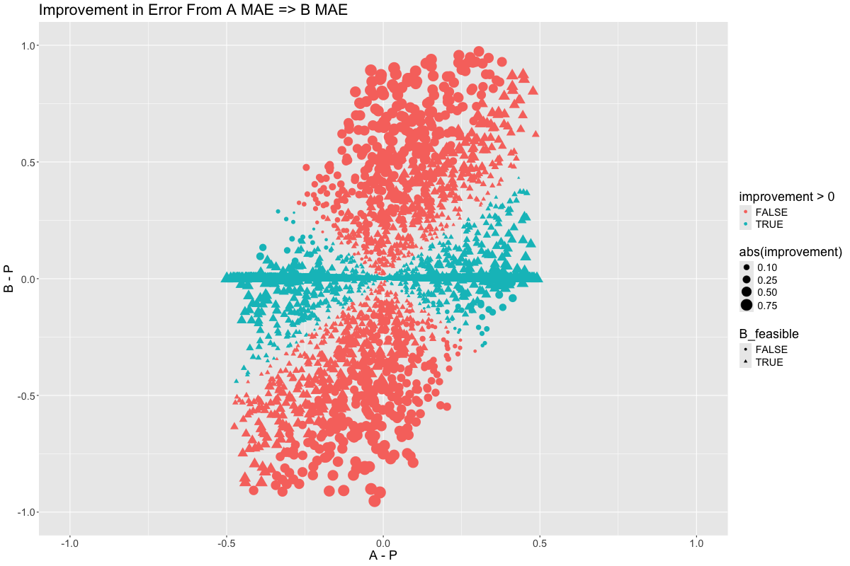
It might make sense to try to understand the trade off between picking \(A\) vs \(B\) as your predictor variable. So let’s sample 4000 trials, and observe the joint distribution of the errors for \(A\) and \(B\):

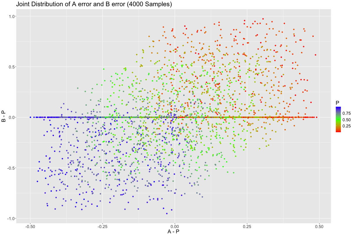
Many trials lie on the x-axis, representing no error with respect to \(B\). This represents instances where our occasionally faulty sensor, \(B\), was not faulty. We see a slight correlation between \(B\)’s error and \(A\)’s error, however. Why is that?

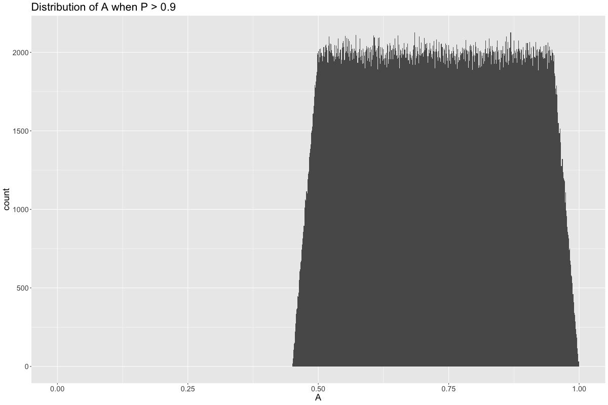
It’s because both \(A\) and \(B\) tend to revert to the mean. That is, whenever \(P \neq 0.5\), both \(A\) and \(B\) will tend to predict a value closer to \(0.5\). For examples, say \(P > 0.9\). What is the distribution of \(B\)?

It is made up of two parts:

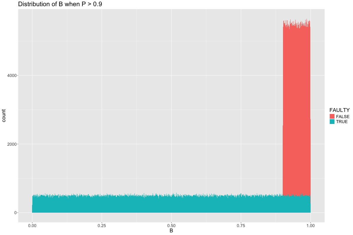
One part is when \(B\) is non-faulty, represented by the red. In these cases, \(B = P > 0.9\). The other part is when \(B\) is faulty, which drags the average of the distribution down from 0.9 and toward 0.5. On the other hand, \(A\) is 50% \(P\) and 50% uniform noise, \(U(0,1)\), and so the distribution of \(A\) is spread out roughly between 0.5 and 1.

If we plot all points of our simulation (when \(B\) is faulty), rather than just 1000 sampled points, then two things become clear:

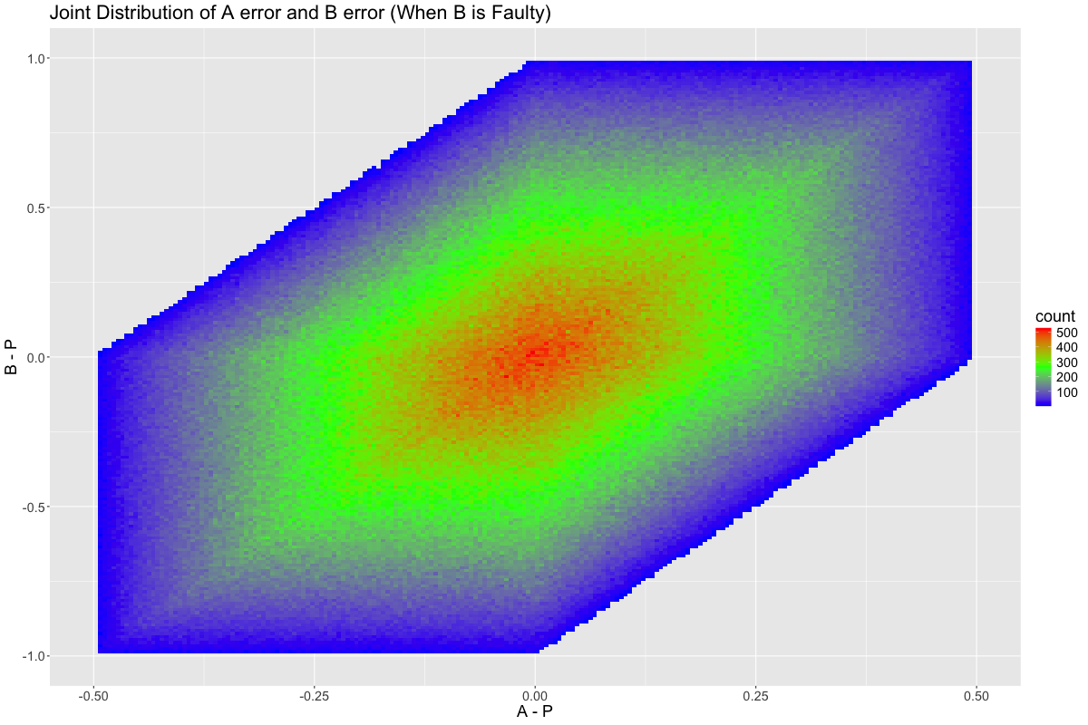
1. Our correlation is quite real
2. There are joint errors that are infeasible

One feature of this problem is that \(B\) has a single huge coin flip. If that coin flip is in our favor, then picking \(B\) is a winning strategy. Otherwise, \(B\) is completely useless to us. Therefore, it might make sense to try to determine if this coin flip landed in our favor.

Consider the case when \(A = 0.9\). What is the distribution of \(B\), both when \(B\) is faulty and when it is correct? It is:

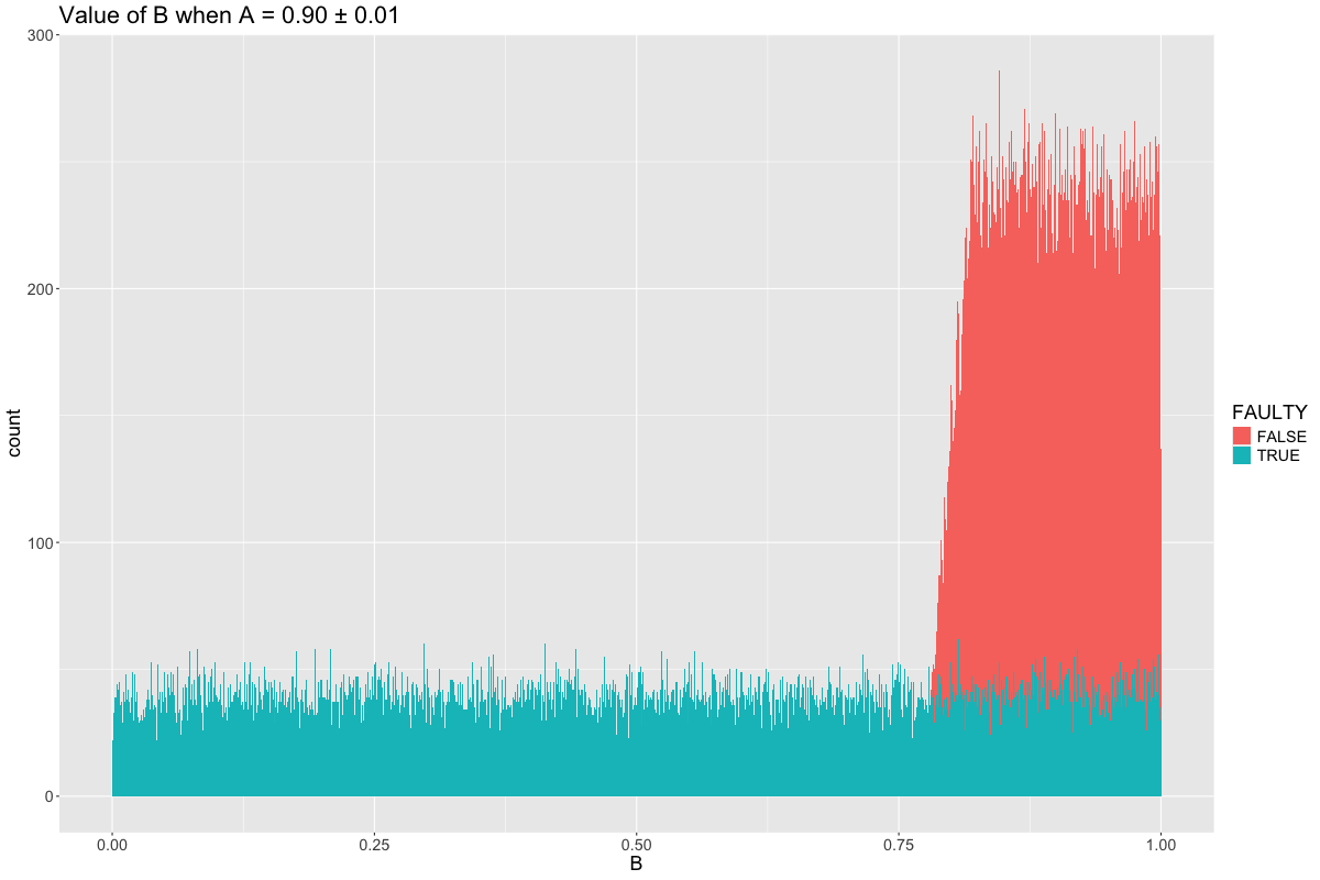
We can see that any value of \(B < 0.8\) must be pure noise. This makes sense, since \(A > 0.9\) implies that \(P\) must be at least 0.8 (since the contribution of \(P\) to \(A\) must be at least 0.4, in addition to a 0.5 contribution from the noise).

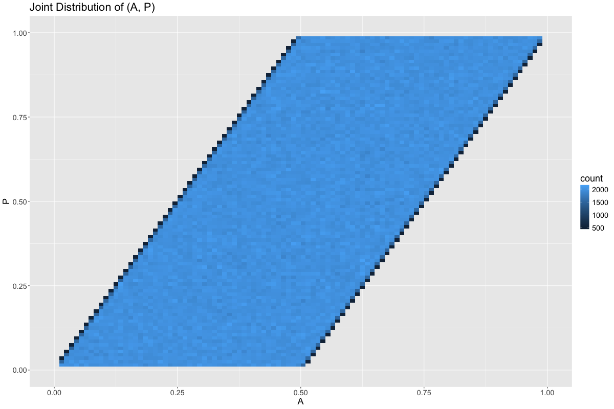
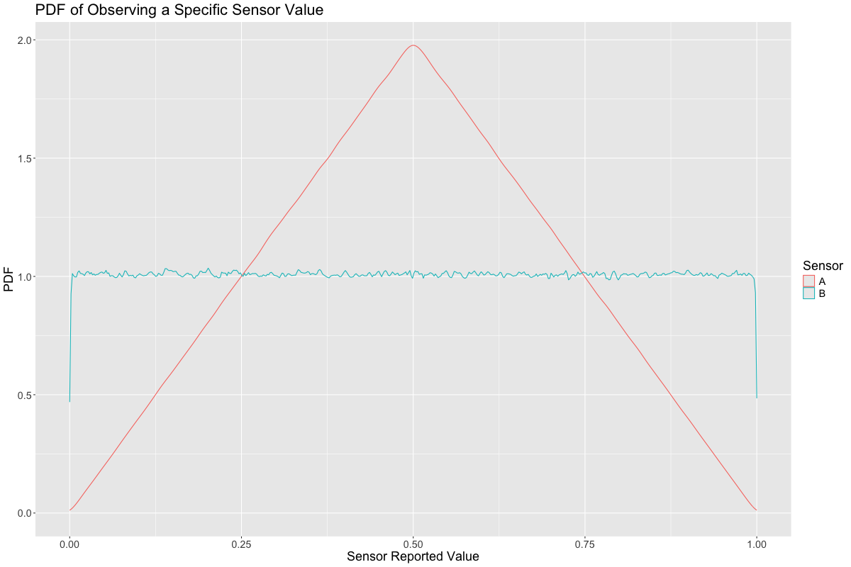
In general, all feasible points in the joint distribution of \(A\) and \(P\) are equally likely:

And the same is true of \((B, P)\), save for \(B = P\):

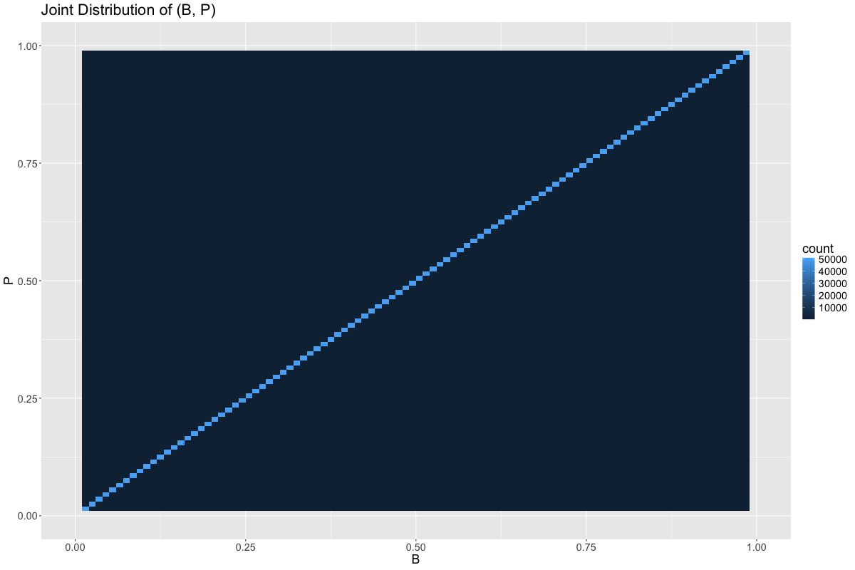
Thus, if \(B\) is feasible, then there is at least a 50% chance that \(B = P\).

So a new strategy emerges:

• If we’re able to determine that \(B\) is pure noise, then the only signal comes from \(A\), making \(A\) the best guess to minimize the L1 and L2 error.
• Otherwise, \(B\) is more-likely-than-not to be the correct answer. Thus, this single point, \(B\), contains more than 50% of the probability mass of \(P\), conditional upon \(A\) and \(B\). Thus, \(B\) is the median of the posterior likelihood function, \(L(P | A, B)\), which makes it the point which minimizes the L1 norm.

Empirically, this gives us a mean absolute error of 0.1041:

|   | name                            | value   |
|---+---------------------------------+---------|
| 1 | 58pct_A_MAE                     | 0.15240 |
| 2 | B_if_feasible_else_A_MAE        | 0.10416 |
| 3 | B_if_feasible_else_A_MAE_from_A | 0.02082 |
| 4 | B_if_feasible_else_A_MAE_from_B | 0.08334 |
| 5 | 58pct_A_MSE                     | 0.03888 |
| 6 | B_if_feasible_else_A_MSE        | 0.00416 |

Credit goes to sweezyjeezy on hackernews. They first presented the proof for this solution.

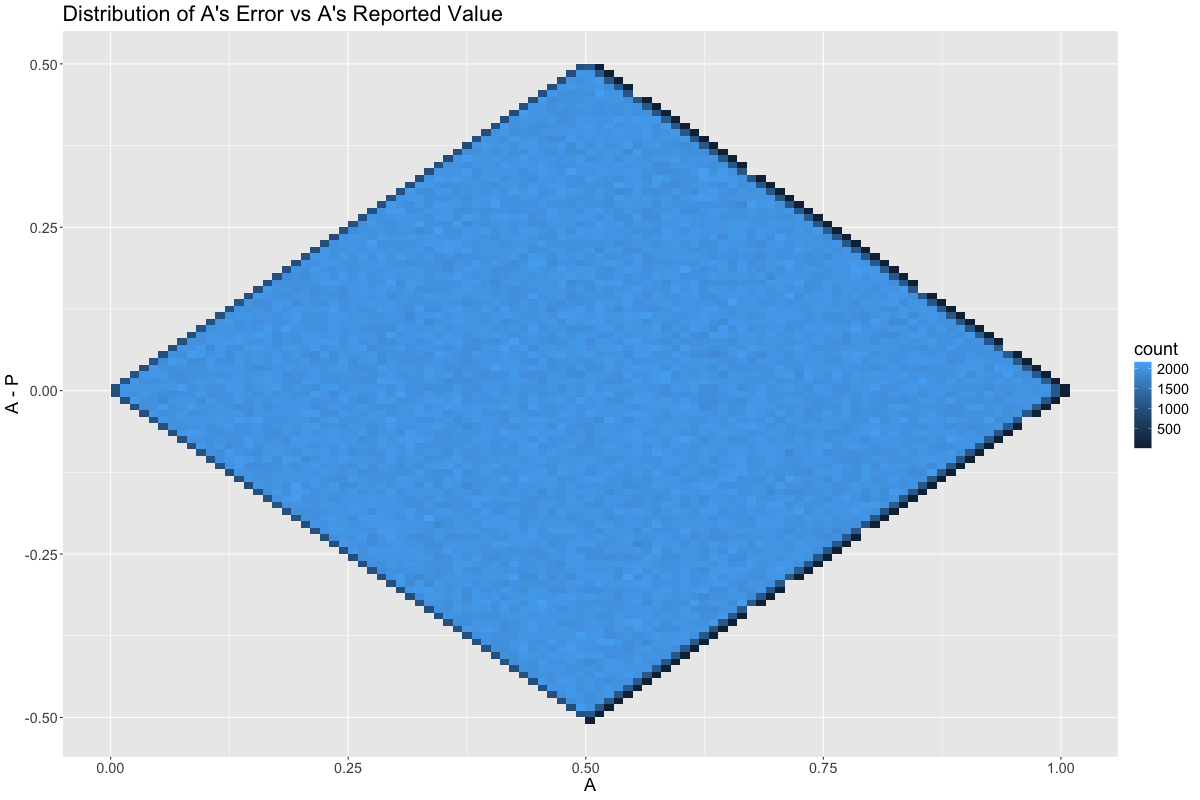
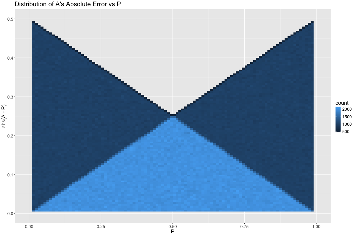
If we plot the distribution of errors conditional upon the value of \(A\), we see that \(A\) is most useful when at the extreme ends of its range. This is because many random noise values are infeasible when \(A\) is near 0 or 1:

Meanwhile, \(A\)’s error is least bad when \(P\) is close to 0.5:

Taking the absolute value of the error from the graph above:

This seems counter-intuitive at first, as we now have two seemingly contradictory statements:

• \(A\), a sensor that reports the value of \(P\), is best when \(P\) is near 0.5
• \(A\) is also best when \(A\) is far away from 0.5

This happens because two things need to align for \(A\) to take on an extreme value. First \(P\) must be large, and second the noise that gets averaged with \(P\) must be large in the same direction. If both of these things happen, then the feasible range of \(P\) is quite small. On the other hand, if only \(P\) is large, then the noise that gets averaged with \(P\) has the potential to be large in the opposite direction, causing a potential error as high as 0.5, e.g., \(P = 1.0\) and the noise is 0.

Contrast this with an observed value of \(A = 0.99\). This observation is actually much more rare, but indicates that both \(P\) and the noise were close to 1.

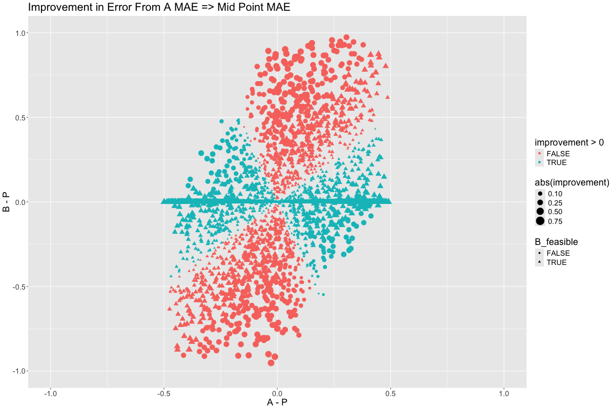
Let’s try to visualize where we’re picking up value when transition from \(A\) toward \(\frac{A+B}{2}\):

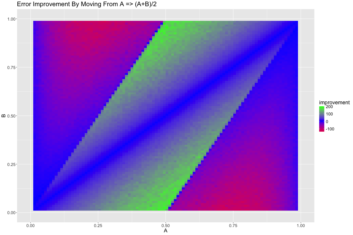
It seems as though the region where \(B\) is feasible is a winner while the region where \(B\) is infeasible is a loser. This makes perfect sense. The line \(A = B\) is neutral because linear combination of two equal terms remains the same, equal, term.

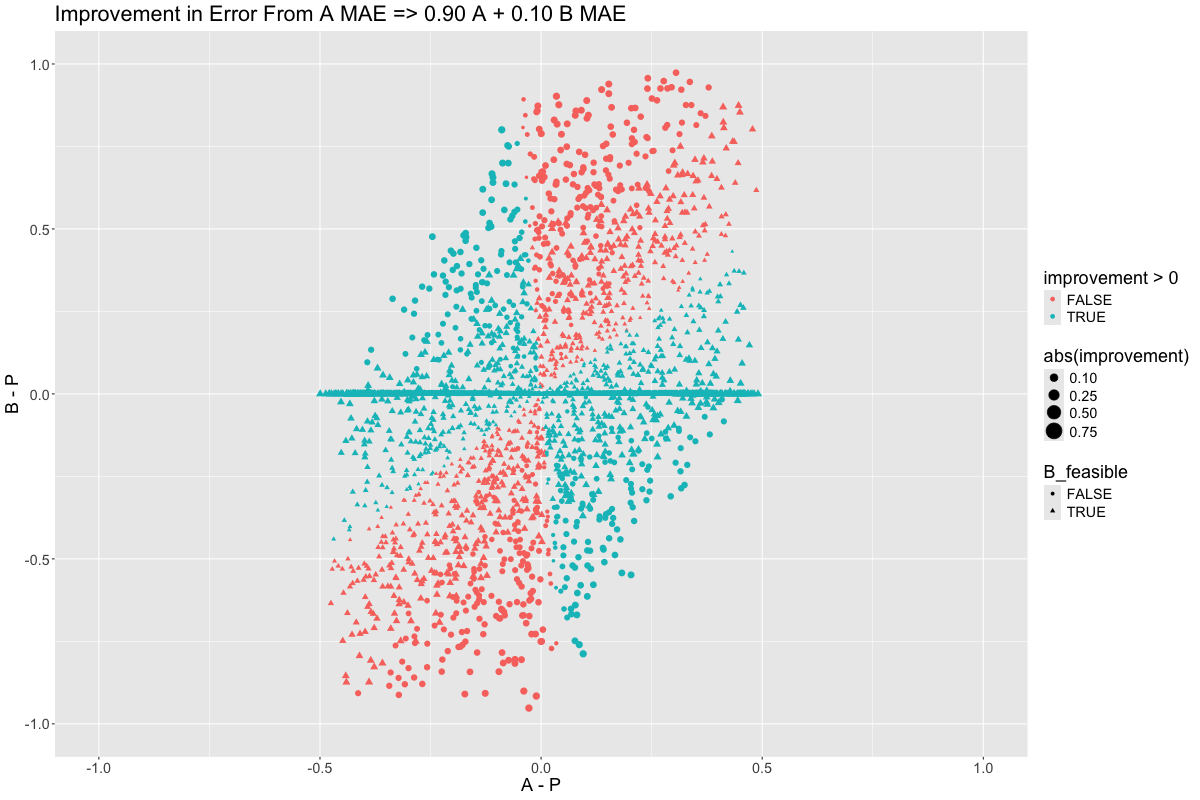
But we know from earlier that we have gone too far in \(B\)’s favor. Lets transition from \(\frac{A+B}{2}\) to \(0.58A + 0.42B\):

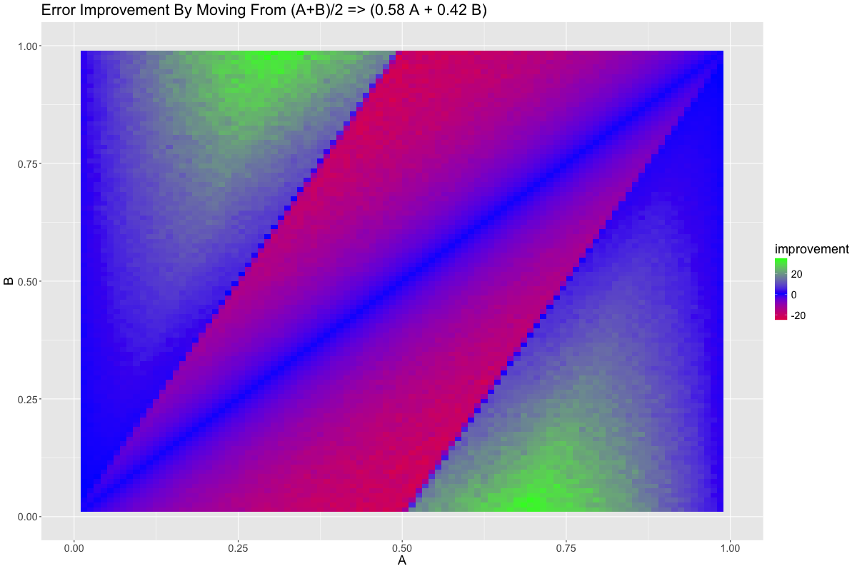
Exactly the opposite, as we would expect. So there is some non-linear term that is causing us to get diminishing returns as we select more and more of \(A\) or \(B\), favoring a balance between the two. What could this be?

We get our first clue when we consider that extreme values of \(A\) decrease the error of \(A\) but extreme values of \(B\) increase the error of \(A\) (since extreme values of \(B\) imply an extreme value of \(P\), which increase the error of \(A\)):

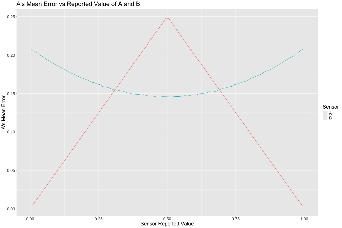
However, in addition to \(A\)’s error getting better at the extremes, the likelihood of observing an extreme value of \(A\) becomes less and less likely at exactly the same rate, while \(B\) is uniformly likely to be observed at any value:

We can reason that points which lie closer to the line \(A - P = -(B - P)\) will benefit most from averaging \(A\) and \(B\) together, because their errors have opposite signs and will cancel. On the other hand, points on the line \(A - P = B - P\) will be unaffected. In general, choosing different linear combinations of \(A\) and \(B\) corresponds to a rotational pattern when we plot the change in the error on the \(A - P\) and \(B - P\) axes:

While I don’t have a closed form solution for why \(0.58 A + 0.42 B\) minimizes the L1 error of all linear combinations of \(A\) and \(B\), it does seem reasonable for a balance to be reached between these two sensors at some place along this rotation. And based on the vertical stretch in the data, I am not surprised that the optimal combination is sightly in the favor of \(A\).